I had used Excel for years earlier than I stumbled throughout most of those options. Like many individuals, I believed I had the appliance fairly properly mastered—shortcuts, formulation, filters, even pivot tables, to not point out the important Excel capabilities each newbie ought to know. However it seems Excel has far more to supply than what you’ll discover in most tutorials.
Likelihood is you haven’t used many of those both, even in case you’d take into account your self an Excel professional. They’re tucked away in menus most individuals by no means contact, which is why they slip underneath the radar. The excellent news is that you simply don’t want superior abilities to make the most of them. A few of these options are simply a few clicks away, but they’ll prevent hours as soon as you understand the place to look.

7
Watch Window
Maintain essential cells in sight with out scrolling
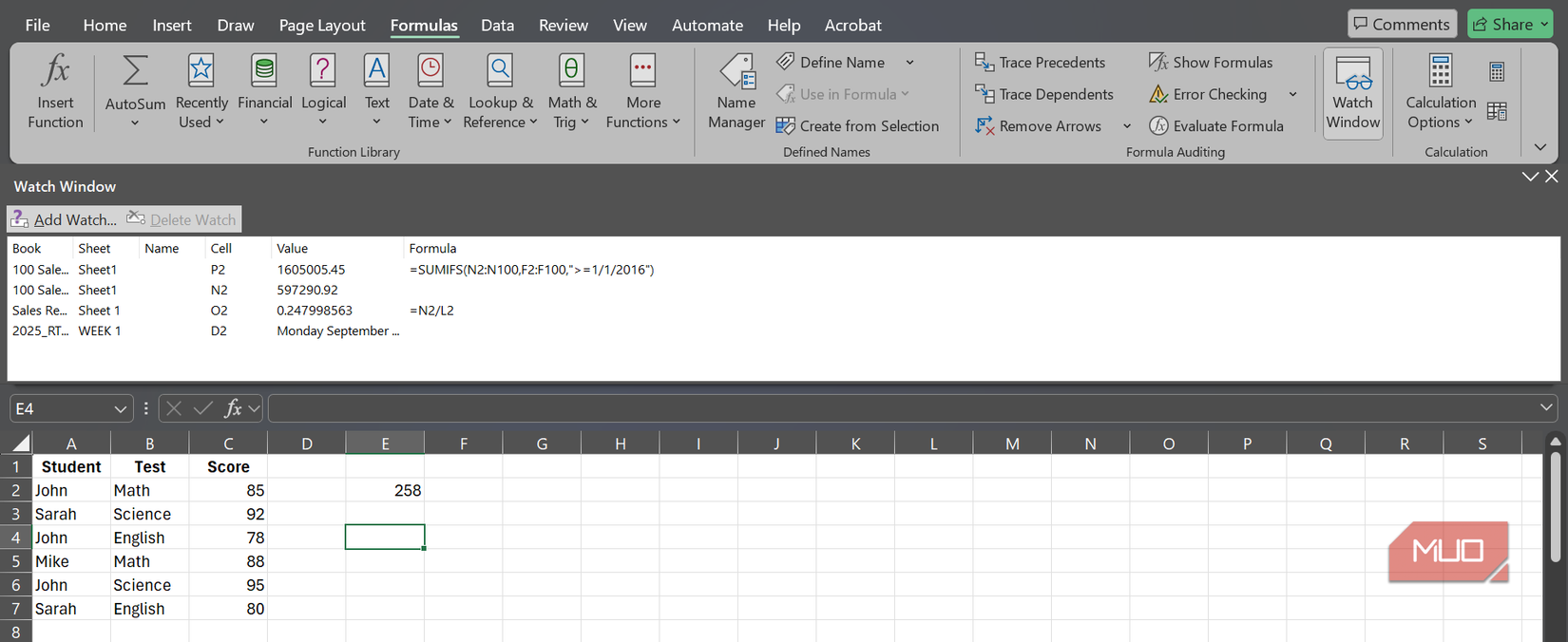
Table of Contents
I used to spend means an excessive amount of time clicking backwards and forwards between sheets, attempting to see how a single change in a single cell affected a number of formulation. It’s so irritating, particularly if you additionally must verify modifications throughout completely different workbooks.
That’s precisely what Excel’s Watch Window is for. It enables you to hold sure cells in view, regardless of which sheet or workbook you’re in, so as to observe key formulation with out infinite scrolling.
You’ll discover it underneath the Formulation tab, within the Method Auditing group. When you open it, simply hit Add Watch and choose the cells you need to monitor. The pop-up will present you the sheet identify, cell reference, present worth, and even the formulation for every cell you’re watching.
By default, it floats in your sheet, however you may dock it underneath the ribbon by double-clicking on the title bar of the Watch Window. Or, in case you’d moderately hold it separate, simply drag it out from underneath the ribbon and resize it nonetheless you want. You’ll discover the expander in case you hover within the backside proper nook of the window.
Whichever means you retain the window in your display screen, you’ll have a continuing dashboard for all of your essential numbers, so that you don’t have to leap between tabs anymore.
Create dwell snapshots of your knowledge
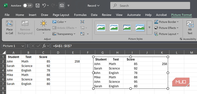
Have you ever ever thought-about a greater means than copying and pasting as a linked image to maintain a clear, always-updating snapshot of your knowledge? The reply is Excel’s Digicam Device. It creates dwell photos of your chosen knowledge ranges, which means the picture updates robotically each time the supply knowledge modifications.
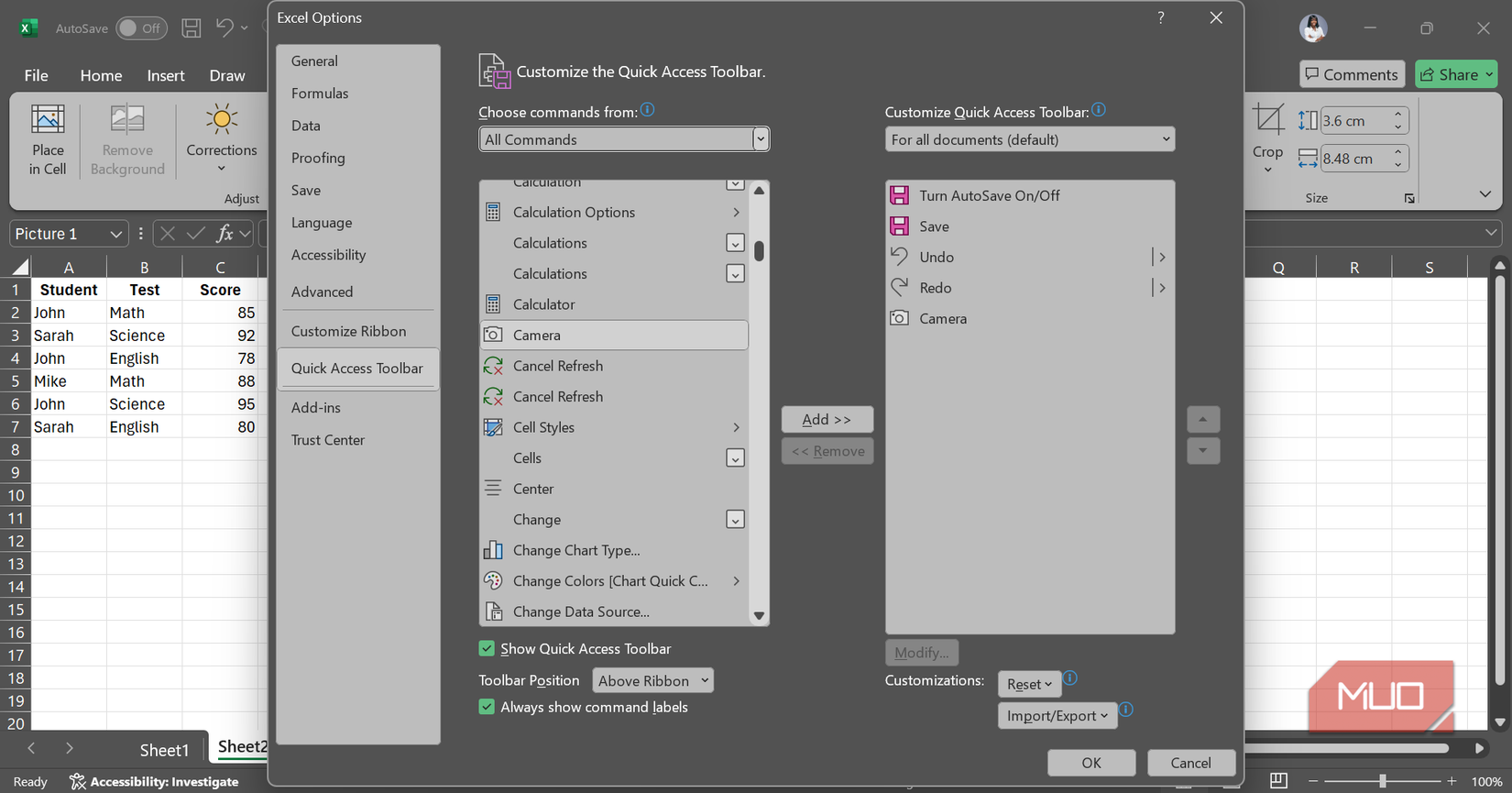
To make use of it, you’ll first want so as to add it to your Fast Entry Toolbar:
- Go to File > Choices > Fast Entry Toolbar.
- Below Select instructions from: choose All Instructions.
- Scroll down, choose Digicam, and add it.
The digicam icon will now seem in your fast entry toolbar, simply earlier than the title of your workbook. To make use of the instrument, spotlight the related cells, click on the Digicam Device, after which click on the place you need your dwell image to seem.
You may even copy the pasted image into Phrase or PowerPoint, though it turns into static outdoors of Excel.
5
Customized Views
Immediately edit your spreadsheet for various audiences
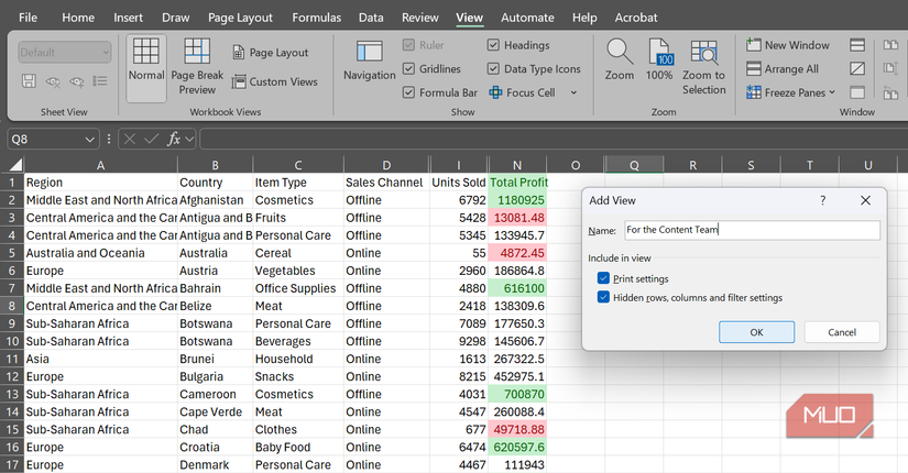
When you’ve ever juggled a number of stakeholders, you understand the battle: advertising and marketing needs one set of columns and filters, finance wants one other, and your boss simply needs a clear model that prints neatly. Sometimes, that might imply both always reformatting the identical sheet or creating separate variations for everybody.
With the Customized Views function, you get another possibility. It enables you to save completely different setups—seen or hidden columns, utilized filters, and even print settings—and change between them immediately. So that you received’t must reformat the identical sheet each time you meet a distinct stakeholder, and also you received’t must create separate variations.
You’ll discover it underneath the View tab within the Workbook Views group. Click on Customized Views > Add and provides your setup a reputation. Often, I’d save my unfiltered and plain sheet as a standard view first. Then, I’d add filters or formatting and save that setup. If I would like one other model, I simply repeat the method with completely different filters or formatting.
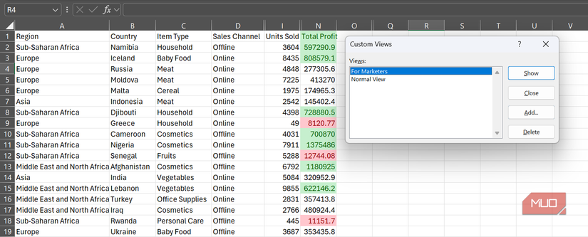
When you’ve saved all of the views you want, it’s only a matter of launching Customized Views, choosing the one you need, and clicking Present.
4
Objective Search
Work backwards to search out the precise enter you want
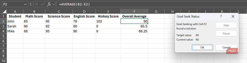
More often than not, we use Excel to calculate outcomes from inputs. When you change the numbers in your sheet, you may see how the result modifications. However what if you understand the consequence you need and want Excel to let you know which enter will get you there?
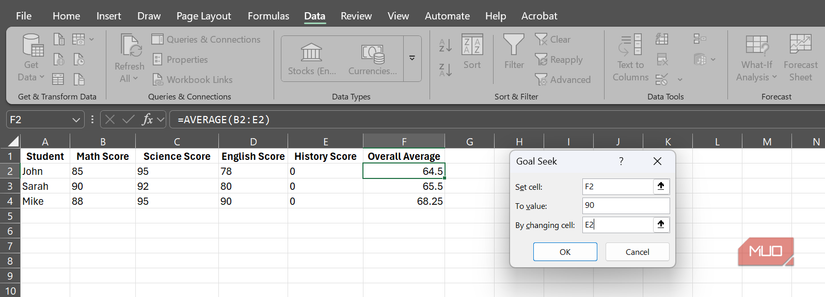
Then, you should utilize Objective Search. It’s Excel’s built-in reverse calculator, and you will discover it underneath the Knowledge tab by clicking What-If Evaluation. Objective Search means that you can set a goal worth for a formulation after which robotically adjusts one enter cell till the formulation reaches that concentrate on.
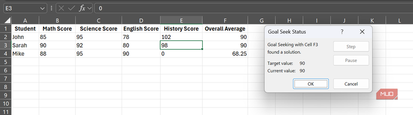
For instance, think about you’ve got a sheet with pupil scores and a last grade calculation, and also you need to know what rating a pupil wants on the ultimate examination (e.g., historical past) to attain a selected total common. As an alternative of guessing and testing completely different values, Objective Search can remedy the issue, so long as it has to do with quantity predictions, in seconds. Merely choose the formulation cell that calculates the general common, set the goal worth (e.g., 90%), and select the enter cell (the rating for the ultimate examination).
When you affirm, Excel will calculate the required rating, and you’ll settle for or reject the consequence.
It’s excellent for locating the numbers you want to obtain a selected purpose, such because the gross sales quantity wanted to interrupt even, the grade required to go a course, or the finances that can hold you on observe.
3
Textual content to Columns
Cut up mixed knowledge into separate columns
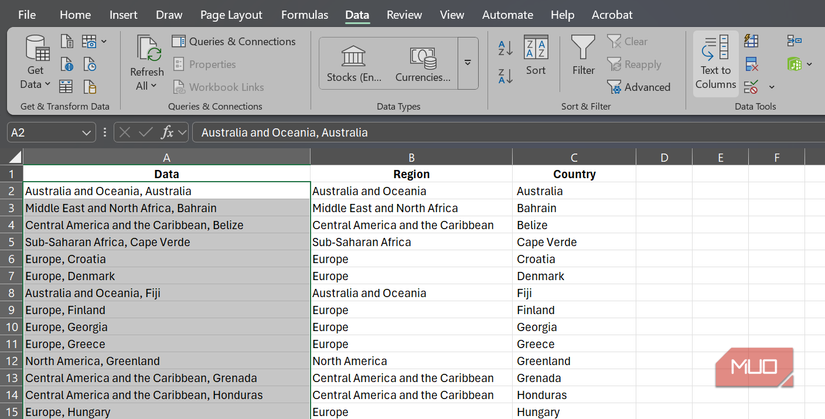
Generally, you import knowledge that leads to a single column when it needs to be unfold throughout a number of columns. When that occurs, the Textual content to Columns function turns into invaluable. It might take the mixed textual content in every column and break up it into a number of columns utilizing delimiters, like commas, areas, and tabs, or mounted widths.
Let’s think about you’ve got a column of places that must be separated into areas and nations. Choose your knowledge column, go to Knowledge > Textual content to Columns, and specify whether or not your knowledge is delimited or fixed-width. Excel will present a preview of the break up and allow you to refine the parameters earlier than making use of the modifications. You may even assign knowledge varieties to every new column in order that dates stay dates and numbers stay numbers.
With only a few clicks, your mixed, messy knowledge will turn into clear, well-formatted knowledge which you can now analyze.
2
Slicers for Tables
Add visible filters to any dataset
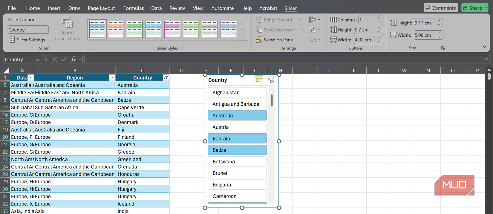
Slicers are sometimes related to PivotTables, however many individuals don’t notice that in addition they work with common Excel tables. As soon as you change a spread right into a desk (Ctrl+T or Insert > Desk), you may add slicers that present the identical intuitive filtering expertise.
To do that, click on wherever inside your desk in order that the Desk Design tab turns into seen, head there, and choose Insert Slicer. You may then select which columns you need to filter by.
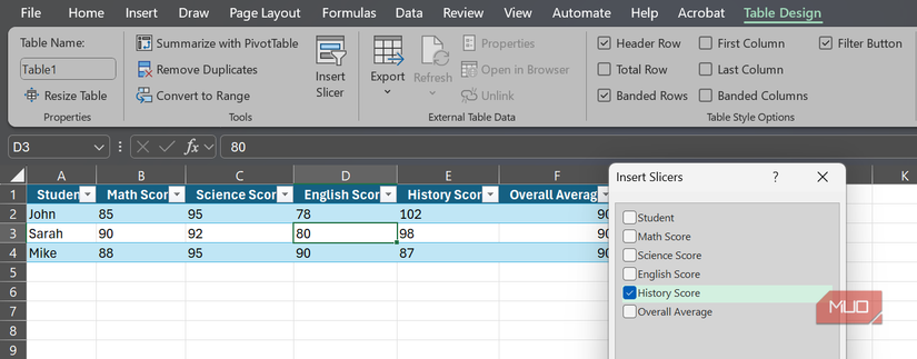
Excel will generate slicer panels for every column, supplying you with buttons you may click on to filter your desk and refine your view immediately.
The slicers additionally spotlight which filters are at the moment utilized, making it a lot simpler than conventional filtering choices to grasp and modify your knowledge at a look.
1
Consider Method
Step by your calculations to debug advanced logic
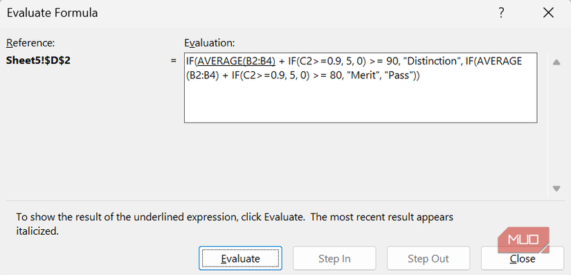
Only a few issues are extra irritating than a formulation returning the flawed consequence, and you’ll’t work out why. You stare at nested capabilities, a number of references, and logical operators, attempting to hint by the calculation mentally. It is like attempting to debug code and not using a debugger.
Excel’s Consider Method enables you to watch a formulation be resolved one piece at a time. Choose the cell with the formulation, go to the Formulation tab, and click on Consider Method within the Method Auditing group.
The dialog highlights the primary a part of the expression; click on Consider to calculate that piece, then proceed stepping by till you attain the ultimate consequence. If the dialog offers the choice to examine a referenced expression, you may step into it (click on Step In) to see how Excel evaluates nested items.
Every step reveals precisely how Excel is deciphering your formulation, which makes it a lot simpler to identify the place a formulation goes flawed. As an alternative of breaking formulation aside or including helper columns, you may watch the calculation occur in real-time.
Every of those seven options has the potential to rework the best way you employ Excel. They aren’t flashy add-ins or superior instruments reserved for specialists, however sensible instruments constructed proper into this system. Whether or not it’s monitoring key values with out scrolling, turning messy knowledge into clear tables, or stepping by a fancy formulation, these options can prevent time and frustration day-after-day.
Begin with one that matches your workflow, and chances are you’ll be stunned at how shortly it turns into a part of your on a regular basis stream.