WRAPCOLS and WRAPROWS Excel are powerful functions that let you reshape your data into columns or rows automatically, saving time and avoiding manual copying.

Table of Contents
Microsoft Excel‘s WRAPCOLS and WRAPROWS functions let you reshape a single row or column of data into a two-dimensional array. This is useful for restructuring raw data, making large datasets easier to read, or creating groups with specific numerical parameters.
At the time of writing (September 2025), the WRAPCOLS and WRAPROWS functions are only available to those using Excel for Microsoft 365, Excel for the web, or the Excel mobile app.

What Are WRAPCOLS and WRAPROWS Excel
Excel’s WRAPCOLS function lets you turn a single column or row of data into a two-dimensional array with a specified number of values in each column.
The syntax for this function is as follows:
=WRAPCOLS(a,b,c)
where
- a (required) is the one-dimensional array (a single column or row of values) you want to turn into a two-dimensional array,
- b (required) is the maximum number of values to return in each column of the result, and
- c (optional) is the value to fill any leftover cells after the wrap has been performed. If omitted, leftover cells are filled with the #N/A error.
If the one-dimensional source array contains blanks, these will be returned as zeros in the result.
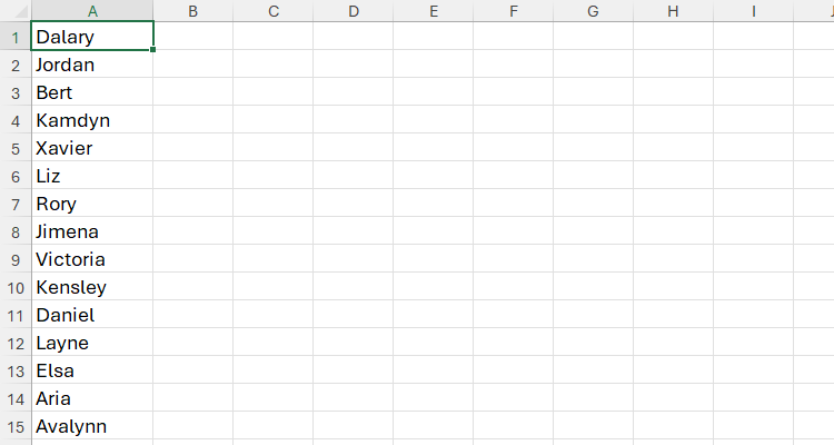
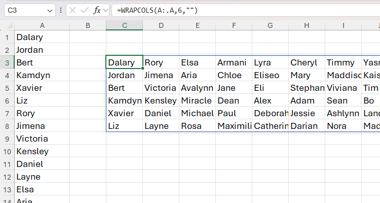
I’ve found this function particularly useful when creating groups from a single list. For example, let’s say you have this Excel worksheet, where cells A1 to A71 contain people’s names, and you want to turn this column into groups with a maximum of six people in each.
To do this, in a blank cell, type:
=WRAPCOLS(A1:A71,6,"")
where
- A1:A71 are the cells containing the one-dimensional array of names,
- 6 tells Excel that the maximum number of values in each column is six, and
- “” tells Excel that any cells left over after the wrap has been performed should be blanks.
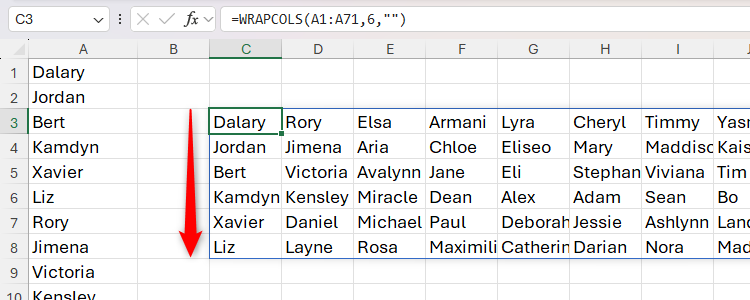
Notice how the WRAPCOLS function keeps the values in their original order down each column. In other words, the six names in the first column are the first six names in the original list, the six names in the second column are the second six names in the original list, and so on.
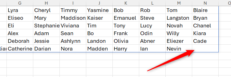
Also, because 71 (the total number of names) isn’t divisible by six (the number of names per group), there are some leftover cells in the result. In this case, they appear blank because the final argument of the formula contains two double quotes.
Another important point to note is that the function generates a dynamic array, meaning the result spills from the cell where you typed the formula to the adjacent cells. This means that if you change the values in the cells referenced in argument a, the result will update to reflect these modifications. However, since dynamic array functions are incompatible with Excel tables, the formula must be typed in a regular cell rather than a table cell.
WRAPROWS: Turning a One-Dimensional Array Into Multiple Rows
Excel’s WRAPROWS function lets you turn a single column or row of data into a two-dimensional array with a specified number of values in each row.
Here’s the WRAPROWS function syntax:
=WRAPROWS(a,b,c)
where
- a (required) is the one-dimensional array (a single column or row of values) you want to turn into a two-dimensional array,
- b (required) is the maximum number of values to return in each row of the result, and
- c (optional) is the value to fill any leftover cells after the wrap has been performed. If omitted, leftover cells are filled with the #N/A error.
Remember that blanks in the one-dimensional source array will be returned as zeros in the result, so you might want to fill these in with an alternative default value first.
Suppose you want to turn this list of names in Excel into seven vertical groups.
To do this, in a blank cell, type:
=WRAPROWS(A1:A71,7,"")
where
- A1:A71 are the cells containing the one-dimensional array of names,
- 7 tells Excel that the maximum number of values in each row (thus, the number of vertical groups) is seven, and
- “” tells Excel that any cells left over after the wrap has been performed should be blanks.
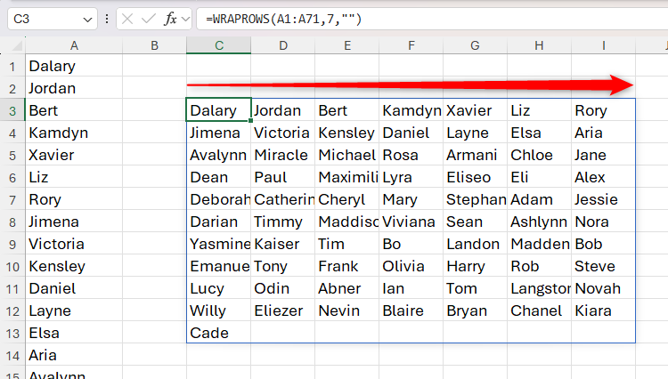
Notice how the WRAPROWS function returns the result in row order, where the first seven names in the source array run across the first row, the second seven names run across the second row, and so on.
Usefully, any changes to the cells referenced in argument a are instantly reflected in the result. However, since WRAPROWS is a dynamic array function, the result cannot be formatted as an Excel table.
Making WRAPCOLS and WRAPROWS More Dynamic
As I’ve already discussed, Excel’s WRAPCOLS and WRAPROWS functions are dynamic, meaning any changes to the original data are reflected in the result. However, making some minor tweaks to their formulas can turn them into truly flexible functions.
There are two potential problems in the straightforward examples above. First, if you add more names to the list in column A, the WRAPCOLS and WRAPROWS functions won’t pick these up, as argument a explicitly references cells A1 to A71. Second, if you wanted to change the number of people in each group, you would need to edit argument b in the formula, a time-consuming process.
Let’s address these one by one.
I’ll use WRAPCOLS in the following examples to demonstrate these processes, but you can apply exactly the same principles to the WRAPROWS function.
Picking Up Additional Values
One way to make the WRAPCOLS and WRAPROWS functions more dynamic is to force them to pick up extra values added to the original one-dimensional array. You could do this by formatting the source data as an Excel table and using a structured reference in the formula.
However, instead of formatting your data, you can reference the whole column and use a trim ref operator:
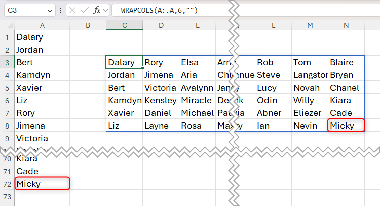
=WRAPCOLS(A:.A,6,"")
where A:.A tells Excel to scan the whole of column A, with the trim ref operator—represented by a single dot after the colon—trimming any blank cells after the last value in the array.
As a result, if you add more names to cells A72 and below, the resultant two-dimensional array picks them up.
Changing the Number of Columns or Rows
Rather than hard-coding the number of values to be returned in each row for argument b, you could achieve the same outcome by referencing a cell.
In this example, cell D1 contains the number six:
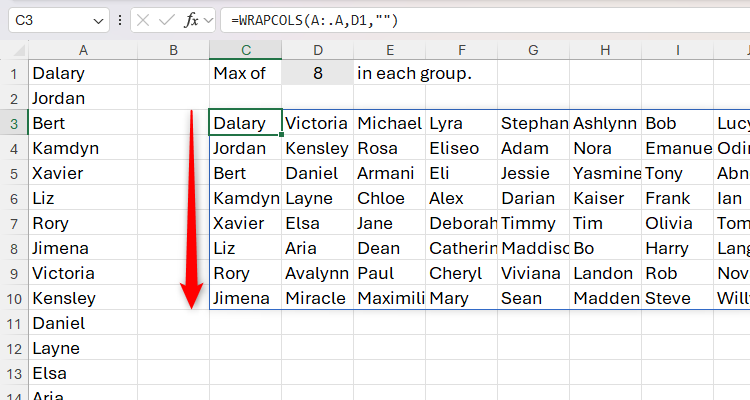
=WRAPCOLS(A:.A,D1,"")
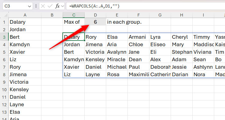
Now, if you want to change the number of people in each group, you can simply alter the value in cell D1.
Adding Dynamic Headers to the WRAPCOLS and WRAPROWS Result
If you’re using the WRAPCOLS function to turn a one-dimensional list into groups, you might consider manually typing column headers—like Group 1, Group 2, and so on—to make the result clearer.
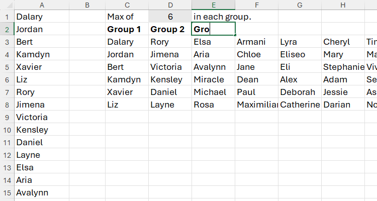
However, a better approach is to enter a formula that creates the column headers automatically, depending on the number of groups created. To do this, you’ll need to use a combination of the SEQUENCE function, the COUNTA function, and the ampersand (&) symbol.
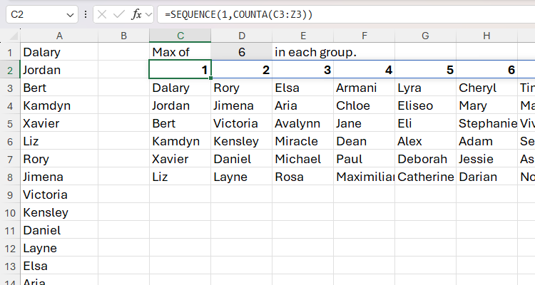
First, use the SEQUENCE function to create a sequence of group numbers:
=SEQUENCE(1,COUNTA(C3:Z3))
where
- SEQUENCE(1…) tells Excel to produce a sequence that occupies one row, and
- COUNTA(C3:Z3) counts the number of non-blank cells from C3 to Z3 to determine the number of columns in the sequence.
Always use dynamic array functions with caution—having too many in one workbook can significantly slow its performance.
That’s great, but what if you want the column headers to have the word Group in them? In this scenario, you can tag this text string to the beginning of the formula:
="Group "&SEQUENCE(1,COUNTA(C3:Z3))
Here, the text string Group—which must be placed inside double quotes—is concatenated to the SEQUENCE formula using the ampersand symbol. I’ve also added a space inside the second double quotation mark so that the word Group is separate from the group number.
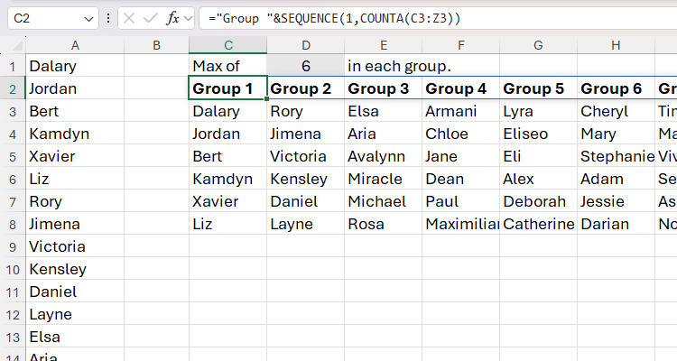
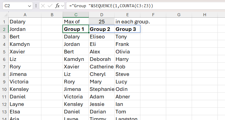
Now, if the number of groups changes, the number of column headers will shrink or grow accordingly.
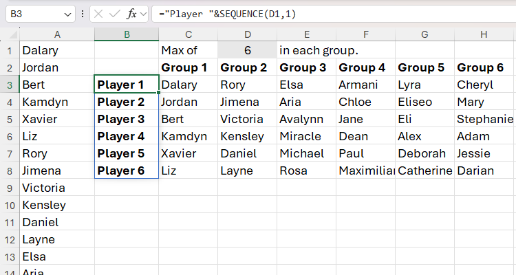
To add row headers to the WRAPCOLS result, you can use a simpler formula:
="Player "&SEQUENCE(D1,1)
In this case, since cell D1 already determines the number of values in each column for the WRAPCOLS function, you can reference the same cell when telling the SEQUENCE function how many rows to occupy. The second argument of the SEQUENCE function is 1 because this is the number of columns you want the sequence to occupy.
Turning Multiple One-Dimensional Arrays Into a Single Two-Dimensional Array
Let’s say you have two lists of names that you want to combine and reorganize into groups of six.
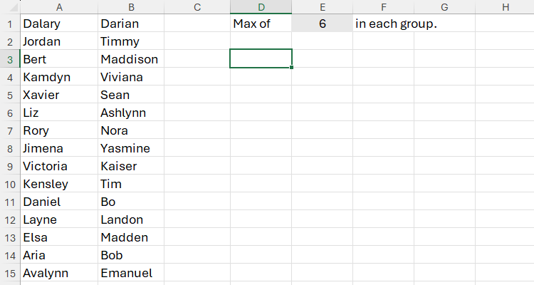
To do this, you need to nest the VSTACK function inside the WRAPCOLS or WRAPROWS function:
=WRAPCOLS(VSTACK(A:.A,B:.B),E1,"")
where VSTACK(A:.A,B:.B) stacks the array in column A on top of the array in column B to create a single list, and the WRAPCOLS part of the formula then turns this single list into a series of columns with six values in each, determined by the value in cell E1.
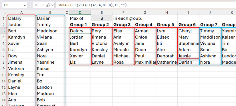
As you can see in the screenshot above, the names from column A, are grouped first, and then the names from column B are grouped immediately after.
On the other hand, if the original lists of names are in separate rows, you can stack these next to each other using HSTACK.
Turning a One-Dimensional Array Into a Sorted Two-Dimensional Array
By default, the WRAPCOLS and WRAPROWS functions return the values in their original order. However, by nesting the SORT function, you can return the values in ascending (alphabetical) order.
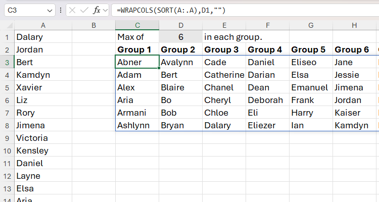
For example, to wrap the array in column A into columns of six, and sort the result from A to Z, type:
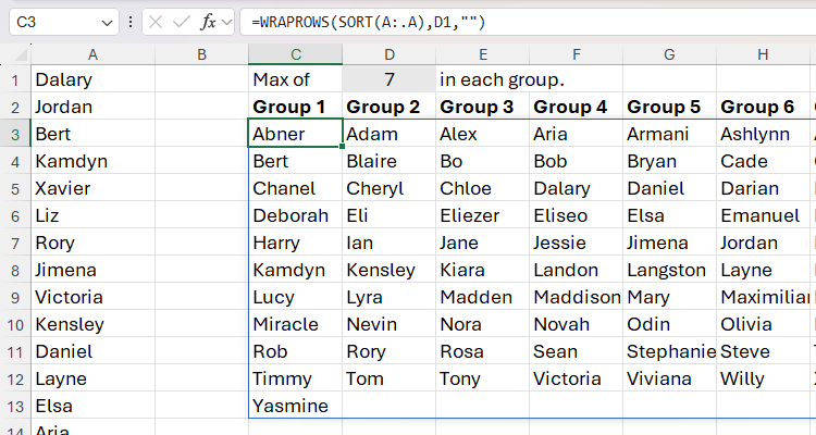
=WRAPCOLS(SORT(A:.A),D1,"")
Similarly, to wrap the array into rows of seven, and sort the output alphabetically by row, type:
=WRAPROWS(SORT(A:.A),7,"")
To sort the values into descending (reverse-alphabetical) order, type -1 for the third argument of the SORT part of the formula, using commas to skip over argument two.
WRAPCOLS and WRAPROWS are not the only ways to reshape data in Microsoft Excel. For example, Power Query lets you flatten your data, PivotTables are great for making large data sets easier to analyze, and the PIVOTBY function allows you to group and aggregate your figures.